White Dwarf Photometric Fit
Photometric fitting can be done by minimizing the \(\chi^2\) with any method supported by scipy.optimize.minimize(), scipy.optimize.least_squares() or with a Markov chain Monte Carlo method powered by emcee (Foreman-Mackey et al. 2013) with the option to refine the solution with minimize() at the end using the 50-percentile as the initial guess and bounding the fit within N-sigmas uncertainty limit (user-defined). The H and He atmosphere type has little effect on the luminosity above around 6000 K. Below this, the assumption of an H atmosphere for an He atmosphere star will lead to an overestimation in the luminosity, and an underestimation in the distance. Optical spectra are not particularly useful in distinguishing the atmosphere type, because below ~5000 K, absorption lines starts to disappear. However, the broad spectral features, namely the collisionally induced absorption, in the infrared can distinguish the atmosphere type (see Figure 12 of Blouin, Kowalski & Dufour 2017). Therefore, readers are reminded to pay particular care when you arrive at a low temperature solution with only optical data. Since it is only possible to fit for \(n-1\) variables, if there are only two photometric bands, it is only possible to fit for a temperature (and luminosity) with an assumed surface gravity and a known distance. With three bands, it is mathematically possible to solve for an extra parameter, i.e. assuming a surface gravity and fit for the temperature and distance, or assuming a distance and fit for the temperature and surface gravity. This argument does not apply to fitting with or without interstellar reddening because it is merely a one-to-one lookup value that is a only a function of distance. When studying a population of WDs that are fitted for the distance, we should compare the photometric distance to the distances measured from other means, e.g. astrometry, spectroscopic distance etc. in order to assess the bias in the fit (e.g. Section 3.2.2 in Rowell & Hambly 2011).
The effective temperature (and absolute bolometric magnitude) and the solid angle of a source can be obtained when the distance is known, through the relation \(\Omega = \pi R^2 / D^2\). In the era of Gaia (Gaia Collaboration et al. 2021), most WDs candidates have their parallaxes measured, and hence the distances derived (Bailer-Jones et al. 2021). This allows much more reliable photometric fitting with broadband photometry alone, as compared to fitting with an assumed surface gravity. By using evolutionary model of WDs, the radius and the effective temperature can be used to obtain the mass (and surface gravity). Even though this is known as the photometric fitting, and values are almost exclusively reported in magnitude, the measurement of the apparent brightness is ultimately performed in electron counts. With good calibration and detector linearity behaviour, it is sufficiently accurate to treat the uncertainties at the flux level. The
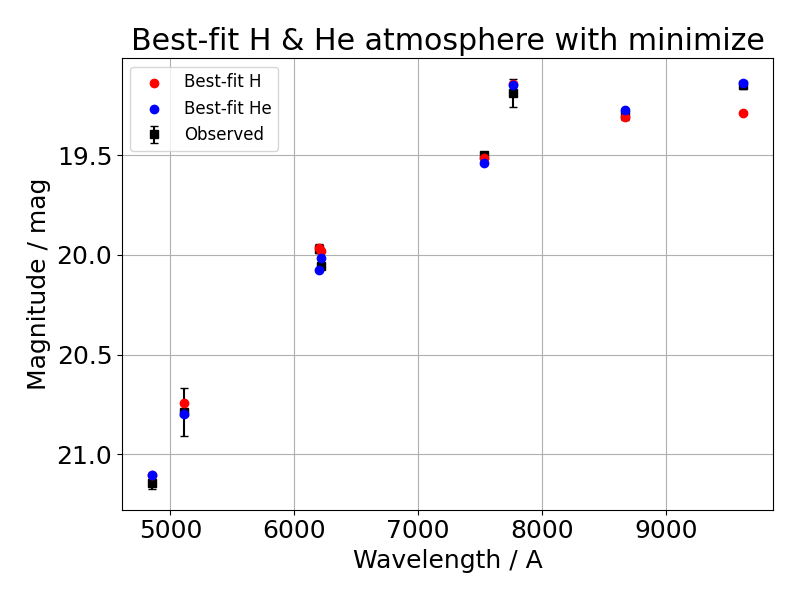
uncertainty in flux measured has a Gaussian-like error that is symmetrical to both over- and under-estimation of the flux. Unlike with magnitudes, which is in the logarithmic space of the flux, the uncertainty in magnitude is no longer symmetrical about the “central” value. Thus fitting directly with magnitude weighted by the magnitude uncertainty leads to a bias: solutions are biased to be over-luminous. For example, at \(\pm0.1\) mag, the flux ratios are 1.0965 and 0.9120, respectively, corresponding the \((-)8.8\%\) and \((+)9.65\%\) change in the flux in the faint and bright end. This only narrows down to \((-)0.917\%\) and \((+)0.925\%\) at \(\pm0.01\,\) mag level [1]. This effect becomes visually obvious if one is to perform an MCMC sampling and inspect the probability distribution functions. For this reason, in WDPhotTools, we fit in flux-space where the linear and symmetrical approximation of the uncertainty distribution is much more realistic. Below is an example diagnostic plot of the photometric fit of the ultra cool white dwarf PSOJ1801p6254.