Model Plotting
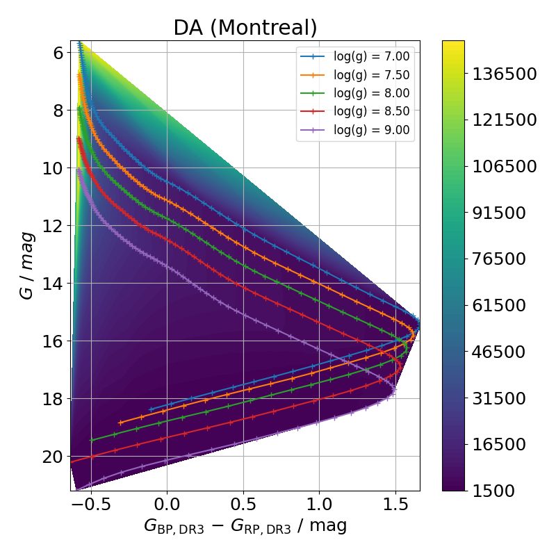
To inspect the Montreal atmosphere models, it can be done easily with the following lines. The following example plots the colour-magnitude diagram in the Gaia eDR3 filters. It can easily be changed to a colour-colour diagram by changing the y=”G3” to, for example, y=”G3-GE_RP”. The available parameters of the model can be retrieved with plotter.list_atmosphere_parameters()
from WDPhotTools import plotter

plotter.plot_atmosphere_model(
    x="G3_BP-G3_RP",
    y="G3",
    atmosphere="H",
    invert_yaxis=True,
    savefig=True,
    folder=".",
    filename="DA_cooling_tracks_from_plotter",
    ext=['png', 'pdf'],
)
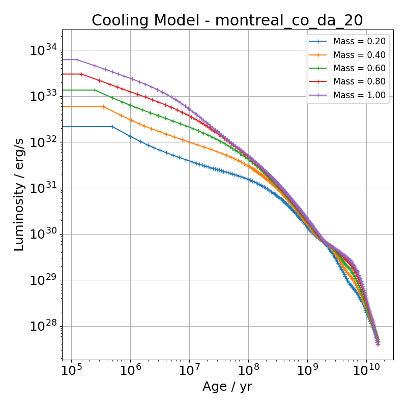
In order to inspect the cooling models, it is slightly less straight forward because each model comes with different parameters. In the following example, we define the model to be montreal_co_da_20 and plotting the cooling tracks at those 5 masses only. The names of the models can be retrieved with plotter.list_cooling_model(), while the model parameters can be found using plotter.list_cooling_parameters(MODEL_NAME)
from WDPhotTools import plotter

plotter.plot_cooling_model(
    model="montreal_co_da_20",
    mass=[0.2, 0.4, 0.6, 0.8, 1.0],
    savefig=True,
    folder="example_output",
    filename="DA_cooling_model_from_plotter",
)
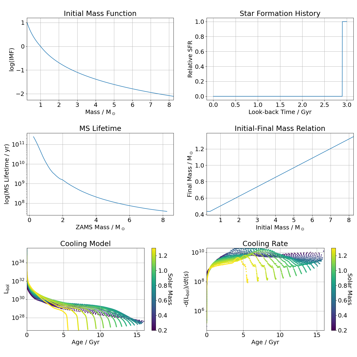
A convenient diagnostic to inspect the input model is available with the WDLF, using the plot_input_models will dispaly a figure with 6 diagnostic subplots: the intial mass function, star formation history, total stellar evolution time, initial-final mass relation, cooling tracks and cooling rates.
import numpy as np
from WDPhotTools import theoretical_lf

wdlf = theoretical_lf.WDLF()

Mag = np.arange(0, 20.0, 2.5)
age = [3.0e9]
wdlf.set_sfr_model(mode="burst", age=age[0], duration=1e8)
wdlf.compute_cooling_age_interpolator()

fig_input_models = wdlf.plot_input_models(
    cooling_model_use_mag=False,
    imf_log=True,
    display=True,
    folder=".",
    ext=["png", "pdf"],
    savefig=True,
)